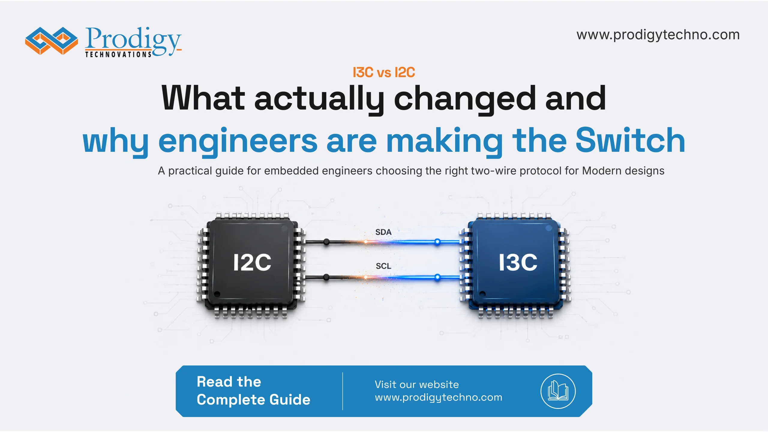
I3C vs I2C: What Actually Changed and Why Engineers Are Making the Switch

Most embedded engineers have lived through this. You’re twelve sensors deep into a design, the bus is clean, and everything communicates well.

But then you add one more device and discover it shares a static address with something already on the board. No workaround is elegant. You’re either adding a multiplexer, pulling address-select pins, or respinning the Printed Circuit Board. 

That friction isn’t all that surprising when you consider where I2C came from. Philips introduced it in 1982 to solve a specific problem. Connecting microcontrollers to peripheral chips without burning through the pin budget. Two wires, shared bus, master-slave simplicity. It worked well enough that the embedded world adopted it widely and kept using it for decades.

But devices got smarter, sensor counts doubled, power budgets tightened, interrupt lines started eating GPIO budget, and I2C’s original assumptions stopped holding  .

I3C is the MIPI Alliance’s answer to that accumulation of friction with faster transfers, dynamic addressing, in-band interrupts, and no pull-up resistors. 

 

What I2C Was Built For, and Where It Started Showing Cracks

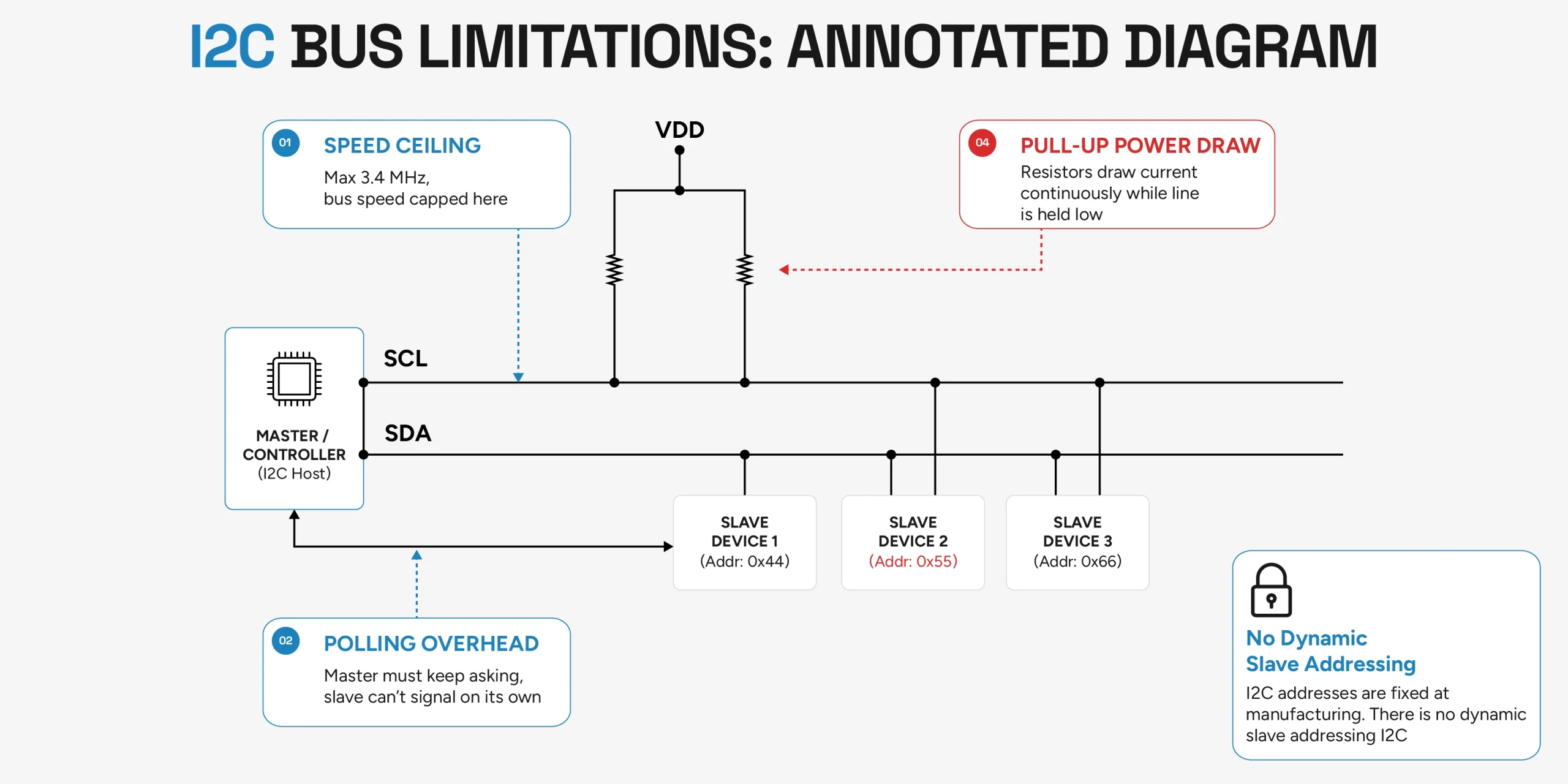
I2C set out to do more with less space and pulled it off. The two-wire bus allowed for simple, clean, and compact board layouts, resulting in more systems with less space. For most of the next four decades, that was enough. Sensors were slow. Microcontrollers were slow. The protocol fit the world it was built for. But ultimately, that changed and the I2C vs I3C debate started. And it’s because of:

• Speed: I2C maxes out at 3.4 MHz in its highest mode. A single temperature sensor has no problem with that. A sensor hub feeding six devices into a fusion algorithm is not. 
• Polling overhead: I2C gives slaves no native way to signal the master. The master has to ask, constantly, burning bus cycles and power even when sensors have nothing new to report.
• Address conflicts: I2C addresses are locked in at manufacturing, and vendors sometimes land on the same address. That causes conflicts when those devices end up on the same bus.
• Pull-up power draw: I2C’s open-drain bus requires external pull-up resistors that continuously draw current during active communication. The higher the bus speed, the stronger the pull-ups need to be. And the more power they consume. 

I3C vs I2C: What I3C Changed and Why

Then came MIPI Alliance with I3C, Improved Inter-Integrated Circuit with the same two pins, higher speeds, low power requirements, and none of the compromises. 

Push-pull signaling

A significant difference between I2C and I3C comes from how the bus is driven. I2C’s open-drain bus can only be pulled low by devices; external resistors do the work of pulling it back high. That passive pull-up is what limits speed and bleeds power. I3C replaces this with push-pull signaling for data transfer. The controller actively drives the bus both high and low. This eliminates the need for pull-up resistors, reduces rise and fall times, and allows for faster data rates and lower power consumption.

Speed

I2C vs I3C data rates is where the comparison becomes clearest. I3C’s Standard Data Rate reaches 12.5 MHz, with High Data Rate modes supporting up to 100 Mbps, far surpassing I2C’s maximum of 3.4 MHz. For the sensor hub that was choking on I2C’s bandwidth, it’s a different operating regime entirely. The bus stops being the issue.

Dynamic addressing

In I2C, two devices with the same hardwired address on the same bus is a hardware problem that requires a hardware fix. I3C solves it in software, at initialization. During Dynamic Address Assignment (DAA), the controller broadcasts an ENTDAA command. Each device responds with its 48-bit unique Provisioned ID, containing vendor ID, part ID, and instance ID, and the controller assigns a unique 7-bit dynamic address to each one.

In-Band Interrupts

To alert the host, a sensor relies on a dedicated interrupt pin on the I2C bus. In sensor-rich designs, this means more traces, more GPIOs, and more interrupt code to manage.

I3C eliminates the extra pin entirely. When a slave has data or an alert to report, it requests control of the bus during an idle period. The controller acknowledges it, and the device sends its dynamic address plus a status byte, all over the same SDA line already used for data. 

When multiple slaves assert IBI simultaneously, the device with the lowest dynamic address wins arbitration.

Backward compatibility

I3C is backwards compatible with I2C devices. I3C controllers can communicate with I2C devices, with the important requirement that legacy I2C devices must have a 50 ns spike filter and must not attempt to hold the clock low (clock stretching), which conflicts with I3C’s push-pull SCL.

Hot-join

With I3C hot-join, new slave devices can be added to a live bus without any interruption in communication. A newly powered device signals its presence using the reserved address 0x02. The controller acknowledges it and runs a DAA sequence to assign a dynamic address.

Here’s a clean comparison of I2C vs I3C protocols across the dimensions that matter most in a real design: 

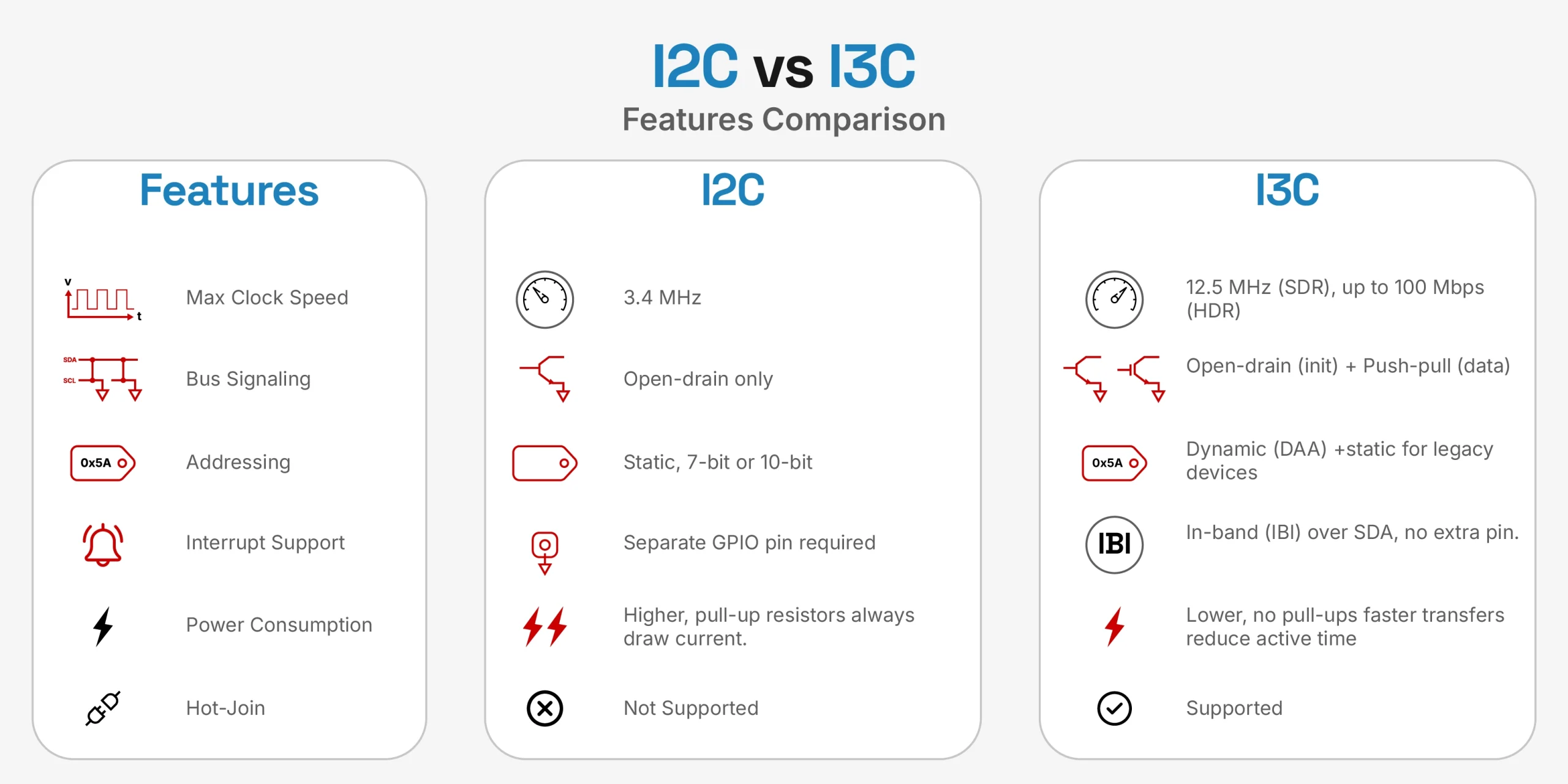
I3C vs I2C: When to Migrate, When to Hold, What the Transition Involves 

Not every design needs I3C because the pull toward new standards is strong and the costs of unnecessary migration are real. Here’s how to think about it.

When you can stay on I2C

• Sensor count is not that high 
• Data rates sit comfortably within Fast Mode Plus
• There’s no pin budget pressure or polling overhead problem
• Power constraints are loose enough that pull-up draw is negligible
• You’re maintaining a legacy system with an established I2C stack

When moving to I3C makes sense

• Address conflicts have already forced multiplexers or board respins
• GPIO interrupt lines are eating your pin budget
• Power is a first-class requirement
• You’re building a platform that will evolve with new sensors across product generations, hot-swap requirements, and modular configurations

What the transition actually involves

Migration from I2C to I3C has several layers.

1. Hardware

Audit every I2C device for clock-stretching behavior. Devices that hold SCL low will conflict with I3C’s push-pull operation and cause bus errors that are hard to diagnose. Also reassess your pull-up resistors; a pure I3C bus doesn’t need them.

2. Firmware

New initialization sequence is the demand of DAA. With IBI, interrupt handling happens through the controller in place of GPIO-triggered ISRs. Your entire I2C driver stack needs rewriting.

3. Tooling

Your I2C analyzer won’t decode DAA sequences or IBI handshakes. Budget for I3C-capable analysis hardware before you start debugging.

 

How to Verify If a Mixed Bus is Behaving Correctly 

A standard I2C analyzer sees the open-drain initialization phase and goes quiet after that. It has no visibility into DAA sequences, IBI handshakes, push-pull data transfers, or HDR mode transactions. A logic analyzer shows you signals and timing, not protocol semantics. Neither tells you why something failed, only that it did. You need a tool that speaks I3C natively, at speed, at the protocol level. 

What to verify

Start with DAA. Capture the full ENTDAA sequence and confirm:

• Every I3C device responds with its correct Provisioned ID
• Dynamic addresses are assigned without collision

Then stress IBI. This is where mixed buses surprise engineers:

• Single device IBI request and acknowledgment
• IBI behavior when the bus is mid-transaction. It should queue, not corrupt

Verify I2C device coexistence:

• Confirm they receive open-drain signaling and respond correctly
• Catch any device attempting clock stretching. 
• Check that I3C high-speed transfers don’t induce glitches on I2C device lines

Finally, validate the electrical layer by checking rise times, voltage compatibility, and bus behavior under thermal and load stress.

The tool that covers all of it

The PGY-I3C-EX-PD from Prodigy Technovations is built specifically for this. It can be configured as an I3C controller, target, or secondary controller. That means you can simulate both sides of any transaction, inject errors, stress the DAA sequence, and validate IBI arbitration without waiting for your hardware to misbehave on its own. 

• It supports legacy I2C devices on the I3C network. You can configure an I3C bus with I2C targets and send I2C traffic to those devices while I3C transactions run alongside. 
• Protocol analysis includes a timing diagram view, protocol listing view, and auto-correlation between the two, so a flagged error in the listing window maps immediately to its position on the waveform.
• Capture is continuous streaming to host storage. For mixed-bus intermittent failures that only surface under sustained traffic, this is the only way to catch them.

Protocol compliance and functional correctness are different things. A bus that passes a quick smoke test but fails under sustained load was never fully verified. The PGY-I3C-EX-PD gives you the visibility to tell the difference. Take a closer look at what it could simplify in your design.