It’s 11 PM and the board on your bench still won’t boot. The MCU has power and the clock is running, but somewhere on the I2C bus, a byte is missing, and you have no clue where.
Twenty years ago, solving this meant walking to a lab that had a logic analyzer bolted to a cart, waiting your turn, and hoping the channel count matched your board. Today it means opening a laptop, clipping a few flying leads onto test points, and watching the bus talk in real time.
That shift, from a shared bench instrument to a personal debug tool, is the story of the logic analyzer.
Why a Logic Analyzer Dominates the Market Today
A logic analyzer captures digital signals. Sorts each sample into a 1 or a 0 based on a threshold voltage. And shows you the result as a waveform or a decoded protocol message. How that job gets packaged is where the three families diverge.
Modular analyzers use a mainframe plus plug-in modules, each module adding a fixed number of channels.
Portable analyzers build everything, screen, controls, processor, into one standalone box. Nothing else is needed to run a capture, but the all-in-one design usually caps performance below what modular gear reaches.
PC-based analyzers, the USB category, strip the box down to just the parts that must sit physically close to the signal like probes, threshold comparators, a sample clock, and the logic that evaluates triggers and packs samples for transmission. Everything else, the display, the storage, the analysis, runs on a laptop that already owns all three.
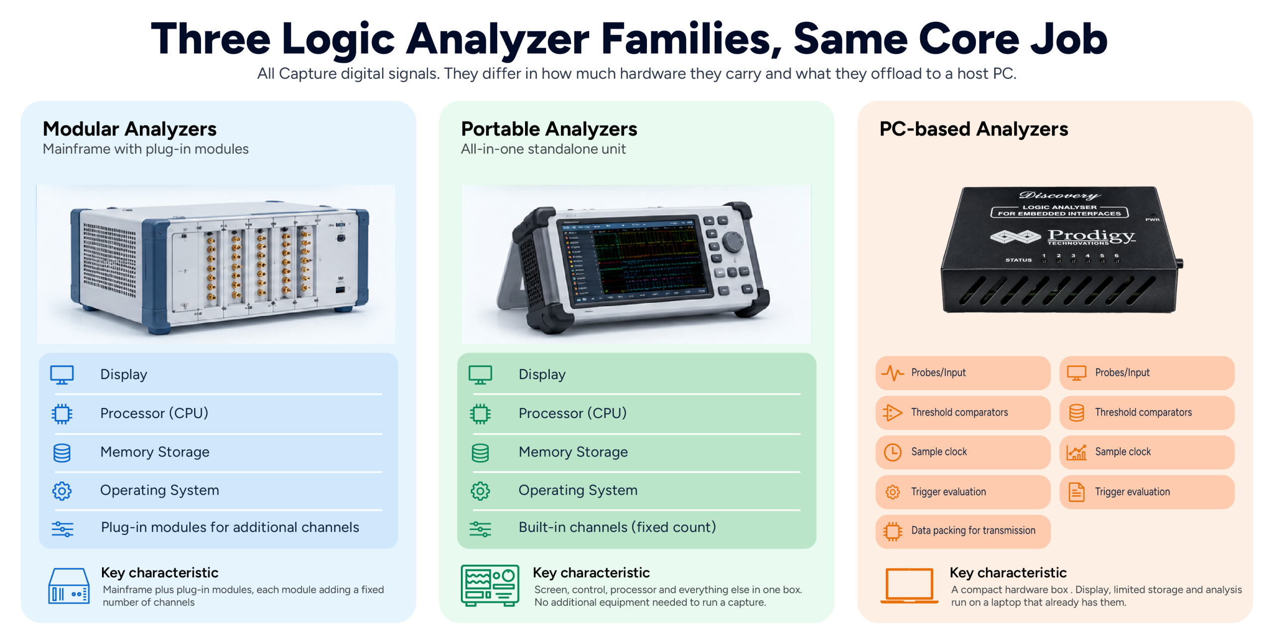
That handoff is the whole reason analyzers took over. A modular or portable unit has to build in a screen, a CPU, memory, and an operating system. A unit doesn’t, because the laptop next to it already has one of each. Skip that hardware and you skip most of the cost and nearly all the bulk.
A few things kept the shift going.
- Supporting a new protocol is now a firmware or software update, not a new circuit board.
- Streaming large captures to a host in real time wasn’t realistic on older interfaces. It is now, and that single change unlocked long, uninterrupted capture sessions.
- Buses like I2C, SPI, and UART, sit comfortably within what a compact USB analyzer handles.
How the USB Interface and Companion Software Work Together
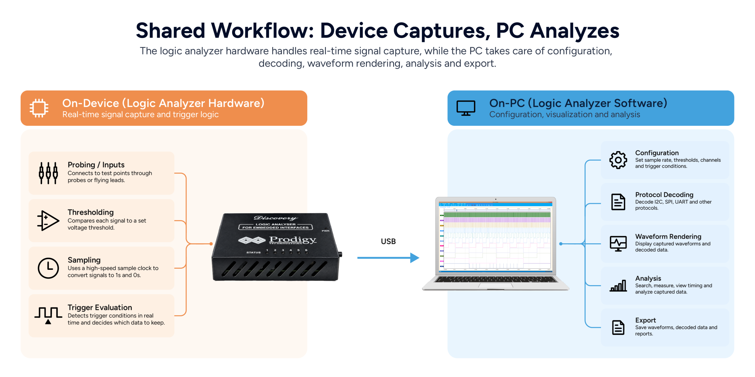
Power line, data channel, and control signal. A single USB cable does all three.
The hardware box takes care of everything that needs to happen at the signal. It connects to the probes, checks whether each signal is above or below the set voltage threshold, and controls the sampling clock. Above the threshold, the signal reads as a 1. Below it, a 0. Everything the analyzer stores comes down to that single decision, repeated millions of times a second.
Configuration lives in logic analyzer software on the PC. You choose the sample rate, set the thresholds, and define the trigger conditions there. But the hardware is what carries them out. Trigger detection in particular has to run on the device in real time, because the analyzer can’t wait for the PC to decide whether a sample is worth keeping. What genuinely happens only on the PC is everything after capture: drawing waveforms, decoding protocols, searching a capture, measuring timing, and exporting a report.
In streaming mode, USB bandwidth becomes a ceiling on what the instrument can do. Each sample on each channel takes up bandwidth on the link, so sample rate and channel count trade against each other. Drop unused channels and the remaining ones can run faster. This is why many software configuration screens ask you to pick channels before they let you pick a sample rate.
Vendors tackle that ceiling in two ways.
In buffered mode, the analyzer stores data in its onboard memory during capture and transfers it to the PC afterward. You get a fixed capture at full speed, which ends when the memory is full.
Streaming mode sends data directly to the PC in real time. That means you can capture much longer recordings. The only catch is that if the USB link can’t handle the data rate, some samples will be missed. It’s the best choice for finding bugs that appear only occasionally.
Capture, Decode, and Trigger Workflow
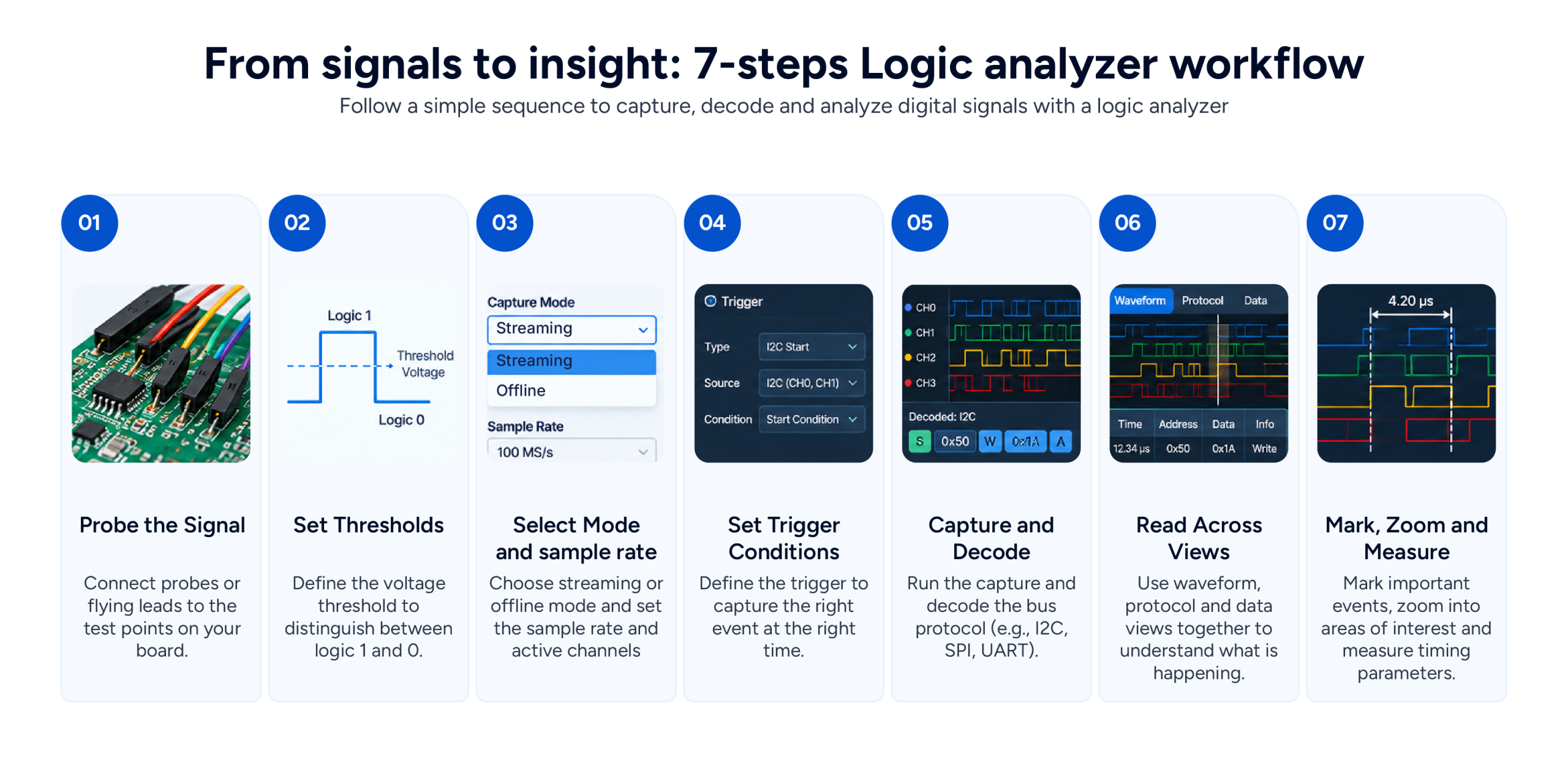 Getting from a bare bus to a readable protocol trace follows a fairly fixed sequence.
- Probe the signal
Clip the flying leads onto the test points. A probe adds its own capacitance and resistance to the circuit under test, and that load can round off sharp edges and slow down transitions. A loose or poorly placed connection produces a capture that looks perfectly clean on screen and is quietly wrong.
- Set the voltage threshold
Tell the analyzer what voltage should count as a logic high. A wrong setting can create false signals or hide real ones.
- Choose the mode and sample rate
Decide whether you need Logic Analysis (LA) mode, Protocol Analysis (PA) mode, or the combined LA + PA Mode, since each frames the same signals differently. Then pick a sampling rate that comfortably outpaces the signal you’re watching. The working rule is at least four times the signal bandwidth, and there is no real penalty for going faster, since a higher sample rate places edges more accurately. Undersampling usually makes a narrow pulse disappear entirely, or show up with the wrong width. A pulse that renders only one sample wide is a warning that you are close to the limit.
- Set the trigger
A trigger defines the condition that starts data capture, so the analyzer records only the event you’re interested in.
Auto captures on any activity, useful for a first look at an unfamiliar bus.
Pattern triggers waits for a specific bit pattern across channels.
Protocol Aware triggers wait for a specific bus event. A START bit, a NACK, a repeated START on I2C, or specific MOSI or MISO data on SPI.
Timing Parameter triggers wait for a pulse or delay of a certain length before capturing data. This helps you catch rare glitches that are easy to miss.
- Capture and decode
Once the raw data is in, the software turns it into readable protocol messages through simultaneous decoding. A design might run I2C, SPI, and UART together, and seeing all three decoded on a shared, time-correlated timeline is what actually reveals whether a delay on one bus is causing a timeout on another.
- Read the result across views
Timing View displays the raw waveforms.
The State or Waveform Listing View shows every captured sample.
The Protocol Decode View interprets the data as protocol packets and highlights errors automatically.
Selecting a frame in the Protocol view auto-correlates back to the exact point in the Timing view, so you’re never manually lining up two windows to find the same moment in time.
- Mark, zoom, and measure
Multiple markers let you tag two points and read the delta between them directly, useful for checking a setup or hold time against a spec. Zoom narrows the view to the exact stretch of signal in question, without losing the wider capture around it.
When to Choose USB Over Modular or Portable
Every debug session doesn’t call for a USB analyzer.
- Choose USB when the work fits a normal embedded bench
Most moderate-speed embedded systems that use I2C, SPI, UART, I3C, or CAN fall within its capabilities. It’s easy to share across a small team and simple to carry to customer sites. USB is also the right call when the fault is intermittent, since streaming capture can run for a long session without a fixed buffer cutting it short partway through.
- Go for portable when the tool needs to stand on its own
Because it runs independently, a standalone unit doesn’t need a laptop. Although it costs more, it’s well suited for field work and secure labs.
- Pick modular when the requirement exceeds what a USB link can carry
USB analyzers are for serial debugging. To validate DDR memory, capture wide buses at high speeds, or run compliance tests, a higher-end analyzer is what you should go for.
For most embedded design work, though, the decision comes down to a short checklist:
- Does the design realistically use more than sixteen to thirty-two channels at once?
- Are you debugging one bus, or several running together?
- Does the analyzer need to leave the lab?
- Is this a shared lab instrument, or a tool that should sit on one engineer’s desk?
If your answers point to a few serial protocols, occasional debugging outside the lab, and a personal tool instead of a shared one, a USB analyzer is the sensible default.
Closing the Loop
Go back to that board refusing to boot at 11 PM. The byte going missing between the sensor and the I2C bus was never really the hard part. The hard part was always visibility, seeing what the bus was doing at the exact moment it went wrong.
That’s the entire case for a logic analyzer. It doesn’t out-muscle a modular chassis on channel count, and it doesn’t try to. It puts a capable instrument exactly where the failure is, running off a laptop that was already going to be there anyway.
For teams juggling several protocols in the same design, I2C, SPI, UART, I3C, SPMI, RFFE, CAN 2.0, and CAN FD, all showing up on the same board, Prodigy’s Discovery series PGY-LA-EMBD is a tool built around exactly that mix. It decodes I2C, SPI, and UART simultaneously in a time-correlated view, across sixteen channels, with 1GS/s timing capture and 100MHz state capture, in a box small enough to travel to wherever the board is. It’s a streaming design, writing continuously to the host drive, which is what makes it a fit for the intermittent fault that won’t repeat on demand.
The byte is still missing somewhere on that bus. The right analyzer is what turns “somewhere” into an address, a timestamp, and an answer.